Simulating the genetic “repressilator”

A demo of an quib-based ODE solver of the classical genetic repressilator.

• Features

  • Quib-linked widgets

  • Running user defined functions using quiby

  • Graphics quibs

  • Graphics-driven assignments

  • Inverse assignments (see the inversion of the log in the Slider value)

• Try me

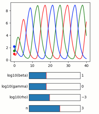
  • Try dragging up and down the circle markers to set the initial conditions of protein concentrations.

  • Try adjusting the sliders to set equation parameters.

Credit

Based on code by Justin Bois, Michael Elowitz (Caltech).

References

• Elowitz & Leibler, A synthetic oscillatory network of transcriptional regulators, Nature, 2000

• Synchronous long-term oscillations in a synthetic gene circuit, Nature, 2016

from pyquibbler import iquib, initialize_quibbler, quiby
initialize_quibbler()
import matplotlib.pyplot as plt
from matplotlib.widgets import Slider
import numpy as np
import scipy.integrate
%matplotlib tk

# Set key parameters:
beta = iquib(10.)
gamma = iquib(1.)
rho = iquib(0.001)
n = iquib(3)  # cooperativity

# time
t_max = iquib(40.)
num_points = iquib(1000)  # Number of points to use in plots
t = np.linspace(0, t_max, num_points)

# Initial condiations (3 x mRNA, 3 x Proteins)
initial_m_x = iquib(np.array([0., 0., 0., 1., 1.5, 2.2]))

# Solver for the mRNA and Protein concentrations
def repressilator_rhs(mx, t, beta, gamma, rho, n):
    """
    Returns 6-array of (dm_1/dt, dm_2/dt, dm_3/dt, dx_1/dt, dx_2/dt, dx_3/dt)
    """
    m_1, m_2, m_3, x_1, x_2, x_3 = mx
    return np.array(
        [
            beta * (rho + 1 / (1 + x_3 ** n)) - m_1,
            beta * (rho + 1 / (1 + x_1 ** n)) - m_2,
            beta * (rho + 1 / (1 + x_2 ** n)) - m_3,
            gamma * (m_1 - x_1),
            gamma * (m_2 - x_2),
            gamma * (m_3 - x_3),
        ]
    )


@quiby
def _solve_repressilator(beta, gamma, rho, n, t, x_init):
    x = scipy.integrate.odeint(repressilator_rhs, x_init, t,
                               args=(beta, gamma, rho, n))
    return x.transpose()

# Run ODE and plot
m1, m2, m3, x1, x2, x3 = _solve_repressilator(beta, gamma, rho, n, t, initial_m_x)

plt.figure(figsize=(4, 3))
plt.plot(t, x1, 'r', t, x2, 'g', t, x3, 'b');

# Plot initial conditions:
plt.plot(0, initial_m_x[3], 'ro')
plt.plot(0, initial_m_x[4], 'go')
plt.plot(0, initial_m_x[5], 'bo');

# Add sliders for parameters
fig = plt.figure(figsize=(4, 2))
axs = fig.add_gridspec(4, hspace=0.7, left=0.3, right=0.8).subplots()
Slider(ax=axs[0], valmin= 0, valmax=3, valinit=np.log10(beta), label='log10(beta)')
Slider(ax=axs[1], valmin=-1, valmax=2, valinit=np.log10(gamma), label='log10(gamma)')
Slider(ax=axs[2], valmin=-5, valmax=0, valinit=np.log10(rho), label='log10(rho)')
Slider(ax=axs[3], valmin= 0, valmax=5, valinit=n, label='n');